Cahn-Hilliard
We prove the existence of a steady-state of the Cahn-Hilliard equation
\[\begin{cases} \partial_t u = -\Delta \left( \frac{1}{\beta} \Delta u + u - u^3 \right), & x \in (0, 1), \\ \partial_n u = 0, & x \in \{0, 1\}. \end{cases}\]
Integrating the steady-state equation twice yields
\[\Delta u + \beta (u - u^3 - c) = 0,\]
where the constant of integration $c$ plays the role of the chemical potential, and $\beta > 0$ is the inverse squared interface width.
Step 1: Formulation
We look for a cosine series solution on $[-1, 1]$.
using RadiiPolynomialF(u, c, β) = Laplacian() * u + β * (u - u^3 - c)DF(u, c, β) = Laplacian() + Multiplication(β * (exact(1) - exact(3) * u^2))Step 2: Approximation (floating-point arithmetic)
The approximate zero
K = 32c, β = 0.0, 40.15625u_init = Sequence(evensym(Fourier(K, π)), [c ; 0.45 ; zeros(K-1)])u_bar, success_newton = newton(u -> (F(u, c, β), DF(u, c, β)), u_init)using CairoMakiefig = Figure()ax = Axis(fig[1,1]; xlabel = L"x", ylabel = L"\bar{u}(x)")lines!(ax, [Point2f(x, real(u_bar(x))) for x = LinRange(-1, 1, 501)]; color = :blue)fig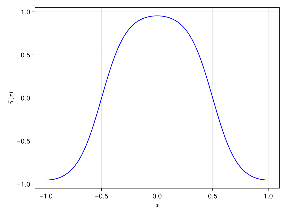
The approximate inverse
struct PseudoInverseLaplacian <: RadiiPolynomial.AbstractDiagonalOperator endRadiiPolynomial.getcoefficient(::PseudoInverseLaplacian, (codom, i)::Tuple{SymmetricSpace{<:Fourier},Integer}, (dom, j)::Tuple{SymmetricSpace{<:Fourier},Integer}) = (i == j) & !(i == j == 0) ? inv(-(frequency(dom) * exact(i))^2) : zero(frequency(dom))Π = Projection(space(u_bar))A_finite = inv(Π * DF(u_bar, c, β) * Π)Step 3: Bounds (interval arithmetic)
using LinearAlgebrac_i, β_i = interval(c), interval(β)u_i = interval(u_bar)A_finite_i = interval(A_finite)Π_i = interval(Π)A = A_finite_i + PseudoInverseLaplacian() * (interval(I) - Π_i)Y = norm(A * F(u_i, c_i, β_i), Ell1())Π_3K = interval(Projection(evensym(Fourier(3K+1, π))))Z₁_finite = opnorm(Π_3K - A * (DF(u_i, c_i, β_i) * Π_3K), Ell1())Z₁_tail = β_i * (interval(1) + interval(3) * norm(u_i, Ell1())^2) / (interval(π) * interval(K+2))^2Z₁ = max(Z₁_finite, Z₁_tail)R = exact(10sup(Y))normA = max(opnorm(A_finite_i, Ell1()), interval(1)/interval(π)^2)Z₂ = exact(3) * β_i * normA * (exact(2) * norm(u_i, Ell1()) + R)ie, success_contraction = interval_of_existence(Y, Z₁, Z₂, R; verbose = true)┌ Info: success: interval found
│ Y = [4.89867e-16, 7.34331e-14]_com
│ Z₁ = [0.0177575, 0.0177576]_com
│ Z₂ = [841.605, 841.606]_com
│ R = ExactReal{Float64}(0.00000000000073433086633548509492733776690906398443813019039083656025468371808528900146484375)
│ Δ = [0.9648, 0.964801]_com
└ roots = ([4.98251e-16, 7.47611e-14]_com, [0.00233421, 0.00233422]_com)Step 4: Conclusion
inf(ie) # smallest error7.476109661219226e-14