• Parameter continuation for the cube root
• • • Step 1: Formulation
    • Step 2: Approximation (floating-point arithmetic)
    • • The approximate zero
      • The approximate inverse
    • Step 3: Bounds (interval arithmetic)
    • Step 4: Conclusion

Parameter continuation for the cube root

We prove the existence of a one-parameter family of solutions to

\[0 = F(u, \lambda) \bydef u^3 - 2 - \lambda, \qquad \lambda \in [-1, 1].\]

Step 1: Formulation

The map $F$ and its derivative $D_u F$ are implemented as follows:

F(u, λ) = u^3 - exact(2) - λDuF(u, λ) = exact(3) * u^2

Consider $[\mathscr{F}(u)](\lambda) = F(u(\lambda), \lambda)$ defined on

\[\mathcal{C} \bydef \left\{ u(\lambda) = \sum_{k \ge 0} (2 - \delta_{0,k}) u_k T_k (\lambda) \, : \, \| u \|_{\mathcal{C}} \bydef \sum_{k \ge 0} (2 - \delta_{0,k}) |u_k| < \infty \right\},\]

where $T_0(\lambda) = 1$, $T_1(\lambda) = \lambda)$ and $T_{k}(\lambda) = 2 \lambda T_{k-1}(\lambda) - T_{k-2}(\lambda)$ are the Chebyshev polynomials of the first kind.

We prove that the quasi-Newton operator

\[G(u, \lambda) \bydef u - A(\lambda) F(u, \lambda)\]

is a contraction near an approximate zero $\num(\lambda) \in \mathbb{R}$ of $F$ for all $\lambda \in [-1, 1]$. Here, $A(\lambda) : \mathbb{R} \to \mathbb{R}$ is an approximate inverse of $D_u F(\bar{u}(\lambda), \lambda)$ for all $\lambda \in [-1, 1]$.

Step 2: Approximation (floating-point arithmetic)

The approximate zero

We use the numerical continuation method to retrieve a numerical approximation of the curve.

We construct a grid of parameters and iterate Newton's method for each step, using the previous approximate zero as the predictor of the solution at the next step.

using RadiiPolynomialK = 10npts = only(grid_size(Chebyshev(K)))λ_grid = [-cospi((j-1)/(npts-1)) for j = 1:npts] # the nodes, swept from λ = -1 to λ = 1u_grid = Vector{Float64}(undef, npts)# initializeu_init = 1.0u_init, success_newton = newton(u -> (F(u, λ_grid[1]), DuF(u, λ_grid[1])), u_init)u_grid[1] = u_init# run continuation schemefor j = 2:npts    w = u_grid[j-1] # naive predictor    u_bar, success_newton_j = newton(u -> (F(u, λ_grid[j]), DuF(u, λ_grid[j])), w; verbose = true)    success_newton_j || error()    u_grid[j] = u_barend# construct the approximationu_cheb = real(to_coef(reverse(u_grid), Chebyshev(K))) # the nodes run from λ = 1 down to λ = -1

Sequence in Chebyshev(10) with coefficients Vector{Float64}:
  1.2410369149251008
  0.1090714005433949
 -0.009688555942404118
  0.0014382541536334613
 -0.0002564899878466125
  5.034289301302231e-5
 -1.0483376552862089e-5
  2.2729343744830322e-6
 -5.087125595069907e-7
  1.2205243614671347e-7
 -2.6866335378628037e-8

The following figure^[1] shows the numerical approximation of the cube root.

using CairoMakiefig = Figure()ax = Axis(fig[1,1], xticks = -3:3)lines!(ax, [Point2f(λ, cbrt(λ + 2)) for λ = LinRange(-3, 2, 501)];    color = :black, label = L"(λ+2)^{1/3}")lines!(ax, [Point2f(λ, u_cheb(λ)) for λ = LinRange(-1, 1, 501)];    color = :blue, label = L"\bar{u}(λ)")scatter!(ax, [Point2f(λ_grid[j], u_grid[j]) for j = 1:npts];    color = :red)axislegend(ax; position = :lt)fig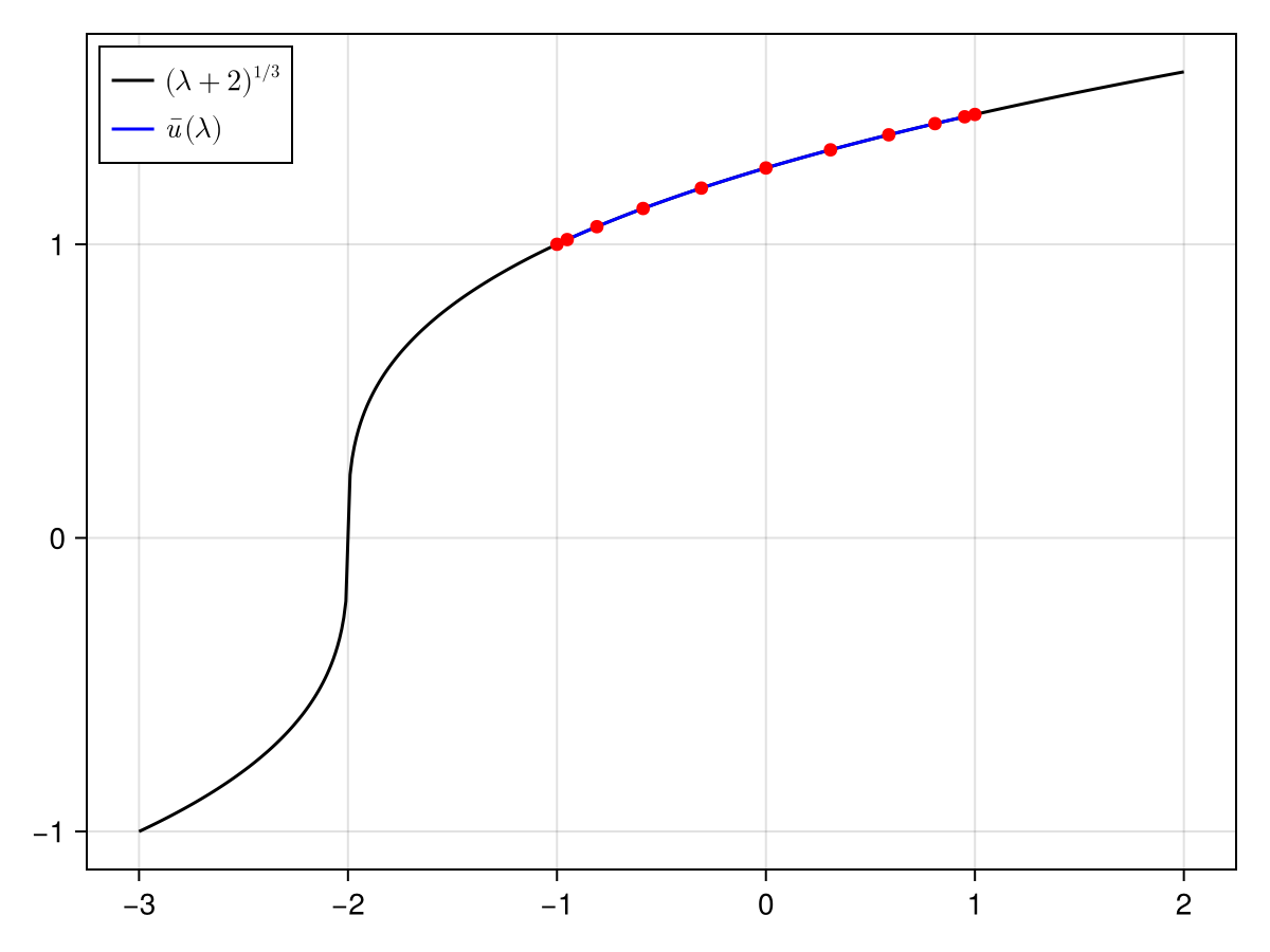

The approximate inverse

We construct the approximate inverse $A(\lambda) \approx D_u f(\num(\lambda), \lambda)^{-1}$ across the continuation branch using standard floating-point arithmetic.

A_grid = inv.(DuF.(u_grid, λ_grid))A_cheb = real(to_coef(reverse(A_grid), Chebyshev(K)))

Sequence in Chebyshev(10) with coefficients Vector{Float64}:
  0.22730980307568133
 -0.040940634509663586
  0.00916700199190223
 -0.002186410752883333
  0.0005374771220529726
 -0.00013449106056040439
  3.404904886402907e-5
 -8.69405259681464e-6
  2.242451106741067e-6
 -6.14893534511829e-7
  1.4924566138496687e-7

Step 3: Bounds (interval arithmetic)

To apply the Radii Polynomial Theorem, we need to theoretically derive and rigorously evaluate the bounds $Y, Z_1, Z_2$. The computer-assisted proof is completed by evaluating these bounds with interval arithmetic:

λ_cheb_interval = interval(Sequence(Chebyshev(1), [0, 0.5]))u_cheb_interval = interval(u_cheb)A_cheb_interval = interval(A_cheb)#- Y boundY = norm(A_cheb_interval * F(u_cheb_interval, λ_cheb_interval), 1)#- Z₁ boundZ₁ = norm(exact(1) - A_cheb_interval * DuF(u_cheb_interval, λ_cheb_interval), 1)#- Z₂ boundR = 10 * sup(Y)Z₂ = exact(3) * norm(A_cheb_interval, 1) * (exact(2) * norm(u_cheb_interval, 1) + exact(R))# verify the contractionie, contraction_success = interval_of_existence(Y, Z₁, Z₂, R; verbose = true)

┌ Info: success: interval found
│ Y = [3.32356e-8, 3.32357e-8]_com
│ Z₁ = [7.08228e-7, 7.08229e-7]_com
│ Z₂ = [2.96414, 2.96415]_com
│ R = 3.323566528905676e-7
│ Δ = [0.999998, 0.999999]_com
└ roots = ([3.32356e-8, 3.32357e-8]_com, [0.674729, 0.67473]_com)

Step 4: Conclusion

For every $\lambda \in [-1, 1]$ there is a solution of $u^3 = \lambda + 2$ within inf(ie) of $\num(\lambda)$, and it is the only one in that ball.

inf(ie) # smallest error

3.323569212704173e-8