The logistic equation

The logistic equation

We prove the existence of a solution of the logistic equation

\[\begin{cases} \displaystyle \dot{u}(t) = u(t)(1 - u(t)), & t \in [-2, 2],\\ u(0) = 1/2. \end{cases}\]

About this example

Proves the solution to $u' = u(1-u)$, $u(0) = 1/2$, on $t \in [-2,2]$.

Involves an infinite-dimensional space: the truncation $\Pi_{\le K}$, the tail $\Pi_{>K}$, and a geometric weight $\nu$.

Assumes Equilibria of the Lorenz system.

Step 1: Formulation

We start by casting the initial value problem into a corresponding zero-finding problem posed on an infinite-dimensional Banach space.

Given $\nu \ge 1$, we consider the Banach space modelling Taylor coefficients of analytic functions on $[-\nu, \nu]$:

\[\mathcal{T}_\nu \bydef \left\{ u(t) = \sum_{k \ge 0} u_k t^k \, : \, \| u \|_{\mathcal{T}_\nu} \bydef \sum_{k \ge 0} |u_k| \nu^k < \infty \right\}.\]

This space is naturally equipped with the Cauchy product $* : \mathcal{T}_\nu \times \mathcal{T}_\nu \to \mathcal{T}_\nu$ given component-wise by, for any $u, w \in \mathcal{T}_\nu$,

\[(u * w)_k \bydef \sum_{l = 0}^k u_{k - l} w_l, \qquad k \ge 0,\]

so that $u(t) w(t) = (u * w)(t)$.

The Banach space $\mathcal{T}_\nu$ is a suitable space to represent a solution of the logistic equation, since it is known that analytic vector fields yield analytic solutions.

It follows that the sequence of coefficients of a Taylor series solving the initial value problem is a zero of the mapping $F : \mathcal{T}_\nu \to \mathcal{T}_\nu$ given by

\[[F(u)](t) \bydef u - \frac{1}{2} - \int_0^t u(s)(1 - u(s)) \, \mathrm{d}s.\]

The mapping $F$ and its Fréchet derivative are implemented as follows:

using RadiiPolynomialF(u) = u - exact(0.5) - Integral(1) * (u*(exact(1) - u))DF(u) = exact(I) - Integral(1) * Multiplication(exact(1) - exact(2) * u)

Consider the fixed-point operator $G : \mathcal{T}_\nu \to \mathcal{T}_\nu$ defined by

\[G(u) \bydef u - A F(u),\]

where $A : \mathcal{T}_\nu \to \mathcal{T}_\nu$ is an operator corresponding to an approximation of $DF(\num)^{-1}$, for some approximate zero $\num \in \mathcal{T}_\nu$ of $F$.

Step 2: Approximation (floating-point arithmetic)

The approximate zero

We numerically compute an approximate zero by performing a finite-dimensional truncation of the problem and iterating Newton's method.

Consider the truncation operator $\Pi_{\le K} : \mathcal{T}_\nu \to \mathcal{T}_\nu$ given component-wise by

\[(\Pi_{\le K} u)_k \bydef \begin{cases} u_k, & k \le K,\\ 0, & k > K, \end{cases} \qquad \text{for all } u \in \mathcal{T}_\nu,\]

as well as the tail operator $\Pi_{> K} \bydef I - \Pi_{\le K}$.

Given an initial guess, the approximate zero is obtained by running Newton's method on the truncated problem, namely $\Pi_{\le K} \circ F \circ \Pi_{\le K}$. For an input u_guess representing an element of $\Pi_{\le K} \mathcal{T}_\nu$, the newton function will automatically perform the truncation $\Pi_{\le K}$:

K = 27u_guess = zeros(Taylor(K))u_bar, newton_success = newton(u -> (F(u), DF(u)), u_guess; verbose = true)

Newton's method: Inf-norm, tol = 1.0e-12, ϵ = 2.220446049250313e-16, maxiter = 15, convergence criterion: |F(x)| ≤ tol
  Iteration       |F(x)|      |DF(x)\F(x)|      ETA (s)
-----------------------------------------------------------
      0      |  5.0000e-01  |  5.0000e-01  |    0.0e+00
      1      |  2.5000e-01  |  2.5000e-01  |    1.7e-03
      2      |  3.1250e-02  |  3.1250e-02  |    1.1e-03
      3      |  1.9531e-04  |  1.9187e-04  |    8.4e-04
      4      |  4.3208e-09  |  4.2857e-09  |    6.9e-04
      5      |  4.2352e-22  |  4.2352e-22  |    5.8e-04

The following figure^[1] shows the numerical approximation in the interval $[-2, 2]$ along with the theoretical solution $t \mapsto (1 + e^{-t})^{-1}$.

using CairoMakiefig = Figure()ax = Axis(fig[1,1], xticks = -5:5, yticks=0:0.25:1)lines!(ax, [Point2f(t, 1/(1+exp(-t))) for t = LinRange(-5, 5, 501)];    color = :black, label = L"1/(1+e^{-t})")lines!(ax, [Point2f(t, u_bar(t)) for t = LinRange(-2, 2, 501)];    color = :blue, label = L"\bar{u}(t)")scatter!(ax, Point2f(0, u_bar(0));    color = :red)axislegend(ax; position = :lt)fig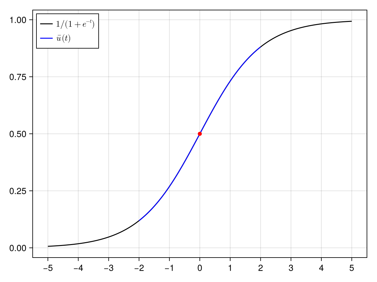

The approximate inverse

We proceed to construct the approximate inverse $A \approx DF(\num)^{-1}$ at the numerical approximation u_bar.

Π = Projection(Taylor(K))A_K_interval = interval(inv(Π * DF(u_bar) * Π))A_tail = interval(I) - interval(Π)A_interval = A_K_interval + A_tail

Step 3: Bounds (interval arithmetic)

Let $R > 0$. Since $T \in C^2(\mathcal{T}_\nu, \mathcal{T}_\nu)$ we use the second-order Radii Polynomial Theorem so that we need to estimate

\[\begin{aligned} Y &\ge \|T(\num) - \num\|_{\mathcal{T}_\nu}, \\ Z_1 &\ge \|DT(\num)\|_{\mathscr{L}(\mathcal{T}_\nu, \mathcal{T}_\nu)}, \\ Z_2 &\ge \sup_{u \in B(\num, R)} \|D^2 T(u)\|_{\mathscr{BL}(\mathcal{T}_\nu, \mathcal{T}_\nu)}. \end{aligned}\]

After some work, we find

\[\begin{aligned} Y &= \|\Pi_{\le 2K+1} A \Pi_{\le 2K+1} F(\num)\|_{\mathcal{T}_\nu}, \\ Z_1 &= \|\Pi_{\le K+1} - \Pi_{\le 2K+1} A \Pi_{\le 2K+1} DF(\num) \Pi_{\le K+1}\|_{\mathscr{L}(\mathcal{T}_\nu, \mathcal{T}_\nu)}, \\ Z_2 &= 2 \nu \max\big( \|\Pi_{\le K} A \Pi_{\le K}\|_{\mathscr{L}(\mathcal{T}_\nu, \mathcal{T}_\nu)}, 1\big). \end{aligned}\]

In particular, since $Z_2$ is independent of $R$, we may freely set $R = \infty$.

The computer-assisted proof leading to the a posteriori rigorous error estimate on u_bar is then completed by evaluating the formulas with interval arithmetic:

u_bar_interval = interval(u_bar)ν = interval(2)X_T = Ell1(GeometricWeight(ν))#- Y boundY = norm(A_interval * F(u_bar_interval), X_T)#- Z₁ boundΠ_Kp1 = Projection(Taylor(K+1))Z₁ = opnorm(interval(Π_Kp1) - A_interval * DF(u_bar_interval) * Π_Kp1, X_T)#- Z₂ boundR = InfZ₂ = max(opnorm(A_K_interval, X_T), interval(1)) * ν * interval(2)# verify the contractionie, contraction_success = interval_of_existence(Y, Z₁, Z₂, R; verbose = true)

┌ Info: success: interval found
│ Y = [1.99289e-6, 1.9929e-6]_com
│ Z₁ = [0.107132, 0.107133]_com
│ Z₂ = [13.7015, 13.7016]_com
│ R = Inf
│ Δ = [0.797157, 0.797158]_com
└ roots = ([2.23205e-6, 2.23206e-6]_com, [0.130328, 0.130329]_com)

Step 4: Conclusion

There is a solution of the initial value problem within inf(ie) of $\num$ in the $\mathcal{T}_\nu$ norm, and it is the only one in that ball. Because $|u(t)| \le \| u \|_{\mathcal{T}_\nu}$ for $|t| \le \nu$, the same number bounds the error on $[-2, 2]$ in $C^0$-norm. Moreover, we have proved that the solution is analytic in $(-2, 2)$.

inf(ie) # smallest error

2.232051998824705e-6

1S. Danisch and J. Krumbiegel, Makie.jl: Flexible high-performance data visualization for Julia, Journal of Open Source Software, 6 (2021), 3349.